Diamonds Forever

Time for a brief personal note. On January 29th 2021, I took the big leap and proposed to my girlfriend, Emma, at L’Auberge Resort in Sedona, Arizona. Thankfully, she said yes and we had an amazing weekend together. This photo below was taken by our photographer minutes after the proposal and captures a moment of pure bliss.

While I could definitely write more about the weekend we had, I am instead going to spend the rest of this post writing about something I wish I had found better information about online before I proposed, diamond engagement rings.

Background

If you are like me when I was going through the process of looking for a diamond engagement ring online, I suspect that at times you will waffle between feelings of extreme uncertainty about what you are purchasing to feelings of extreme blasè or as Drake says, YOLO. The advice I seemed to collect from chatting with most of my engaged or married friends was, learn the 4 Cs (Cut, Color, Clarity, Carat) and to quote my friend Catherine, “if you love her, spend all your money”. While this is sage advice and I did eventually purchase a ring – I won’t disclose from where or how much I spent – I was left wanting for more in-depth information about what diamonds cost and a better explanation why. Lo and behold, here we are.

My strategy for figuring out why diamonds cost what they do in two parts:

1. Scrape a ton of diamond data from popular online engagement ring sites
2. Build predictive models to ascertain what features are most important to diamond price

Disclaimer The rest of this post will focus on understanding diamond price. While, rings and settings are still important and a decent chunk of change, the vast majority of most engagement rings is the diamond gemstone and settings are easier to understand and price compare.

Digging for Diamond Data

Apparently there is already a well known public diamond dataset that is used frequently by the data science community. The popular python visualization package, Seaborn, installs with the diamonds dataset by default. I probably could have saved myself a lot of time by making use of the public dataset, but I do not feel that the data accurately represents the diamonds and prices that I came across when I myself was looking at diamonds online.

My approach then was to pull diamond data from three of the largest online diamond engagement ring sites:

• Blue Nile
• Brilliant Earth
• James Allen

If you were to scroll through each of these sites, you will likely find that they all have a very similar UX flow. In fact, I wouldn’t be surprised if the same third party company designed the “diamond search” feature of all of their websites. My original thought was to try to use Selenium, a web acceptance testing framework that is also useful for manipulating DOM objects and web scraping. Spending maybe 1 or 2 days mucking about with Selenium, I came to the conclusion that the dynamic html tables I was trying to manipulate were too complex and the technique I opted for instead was look through the network calls being made in a development window until I found the call to XYZ’s website backend that was returning the data. Next, I simply used python’s request library to send repeated calls to each websites backend while I manipulated the carat parameter in the request query parameters in order to steadily return different result sets.

NOTE!!! DO NOT. I repeat, DO NOT, mimic this method if you share an IP address with your fiancè to be and/or are not making these requests behind a VPN. For about a month, any and all programmatic advertising I saw was for diamond engagement rings. Because I had started collecting the data before I had been able to propose, I then had to live in constant fear that Emma would grow suspicious of all the diamond advertising she was seeing.

After a big some data cleaning and minimal munging – James Allen uses different labels for cut compared to Brilliant Earth for example – I was left with a (576820, 9) dataset that looked something like this:

1
2
3
4
5
6
7
8
9

print(diamond_df.sample(n=5, random_state=0).to_markdown())

|        | shape    |   price |   carat | cut         | color   | clarity   | vendor          | is_lab   |   log_price |
|-------:|:---------|--------:|--------:|:------------|:--------|:----------|:----------------|:---------|------------:|
|   6412 | Round    |     740 |    0.3  | Ideal       | F       | SI1       | Brilliant Earth | False    |     6.60665 |
|  34866 | Round    |    1110 |    0.4  | Ideal       | F       | SI1       | Brilliant Earth | False    |     7.01212 |
| 164602 | Round    |    2020 |    1.2  | Super Ideal | J       | VS1       | Brilliant Earth | True     |     7.61085 |
|  45097 | Marquise |    1220 |    0.5  | Good        | H       | SI1       | Brilliant Earth | False    |     7.10661 |
| 481003 | Round    |    3720 |    1.04 | Very Good   | F       | I1        | James Allen     | False    |     8.22148 |

Here is an interactive plot showing carat and log price grouped by vendor and whether or not the diamond is a “loose” diamond or a lab diamond.

What the hell are lab diamonds any way?

Lab diamonds are real diamonds, full stop. In fact…

In July 2018, the U.S. Federal Trade Commission approved a substantial revision to its Jewelry Guides, with changes that impose new rules on how the trade can describe diamonds and diamond simulants.[120] The revised guides were substantially contrary to what had been advocated in 2016 by De Beers.[119][121][122] The new guidelines remove the word “natural” from the definition of “diamond”, thus including lab-grown diamonds within the scope of the definition of “diamond”. The revised guide further states that “If a marketer uses ‘synthetic’ to imply that a competitor’s lab-grown diamond is not an actual diamond, … this would be deceptive."[1][121]

Lab diamonds that are used as gemstones are produced using CVD (Chemical Vapor Disposition) or HPHT (high-pressure high-temperature) methods and only recently, as of mid 2010s, have begun to penetrate the gemstone market as upstarts such as Brilliant Earth have entered the market. Gem-quality diamonds grown in a lab can be chemically, physically and optically identical to naturally occurring ones. Also because of awareness that traditional diamond mining has led to human rights abuses, lab grown diamonds are also an ethically sound alternative to “loose” diamonds.

…anyways…back to the data.

Linear Model

One obvious way to try to get a sense of what features have the greatest impact on diamond price is to run a simple linear regression using the natural logarithm of price as a dependent variable. Why log transform your dependent variable you might say? The short answer here is that you always want to avoid skewed distribution in the residuals. By using a log transformation, we are reducing skewness in our dependent variable and approximating a normal distribution thus helping to alleviate this risk. An additional benefit of using the natural log to transform our dependent variable is that it makes interpretation of the coefficients relatively straightforward as a coefficient of .15 equates to a percentage increase of (exp(.15) - 1) * 100 in our dependent variable:

1
2

In [10]: (math.exp(.15)-1)*1e2
Out[10]: 16.183424272828304

So in the example above, our .15 coefficient equates to a ~16.2 % increase in our dependent variable. Ohh….one more thing…there are a lot of categorical variables involved in this dataset: color, clarity, cut, etc. In order to better handle for these, I’ve done one-hot encoding to turn these into dummy variables. Also, because we know that some of these categorical dummmies are perfectly correlated with each other, if a diamond is color E it cant also be color F, I’ve removed the following columns ['Fair', 'K', 'I1' , 'Blue Nile','Emerald', 'price'] from the datatset and added a constant term. Because we’ve removed the above dummmies, the constant in the regression results below captures the variance for a Fair cut, K colored, I1 clarity, Blue Nile emerald shaped diamond.

 1
 2
 3
 4
 5
 6
 7
 8
 9
10
11
12
13
14
15
16
17
18
19
20
21
22
23
24
25
26
27
28
29
30
31
32
33
34
35
36
37
38
39
40
41
42
43
44
45
46
47
48
49
50
51
52
53
54
55
56

                            OLS Regression Results                            
==============================================================================
Dep. Variable:              log_price   R-squared:                       0.831
Model:                            OLS   Adj. R-squared:                  0.831
Method:                 Least Squares   F-statistic:                 7.073e+04
Date:                Thu, 18 Feb 2021   Prob (F-statistic):               0.00
Time:                        07:08:13   Log-Likelihood:            -2.6180e+05
No. Observations:              461453   AIC:                         5.237e+05
Df Residuals:                  461420   BIC:                         5.240e+05
Df Model:                          32                                         
Covariance Type:            nonrobust                                         
===================================================================================
                      coef    std err          t      P>|t|      [0.025      0.975]
-----------------------------------------------------------------------------------
const               5.1746      0.020    254.261      0.000       5.135       5.214
carat               1.6968      0.001   1440.295      0.000       1.695       1.699
is_lab             -0.8574      0.002   -426.629      0.000      -0.861      -0.853
Asscher             0.0757      0.014      5.434      0.000       0.048       0.103
Cushion             0.0953      0.007     13.902      0.000       0.082       0.109
Heart               0.1861      0.012     15.468      0.000       0.163       0.210
Marquise            0.1919      0.010     19.611      0.000       0.173       0.211
Oval                0.1430      0.005     27.629      0.000       0.133       0.153
Pear                0.1833      0.006     31.382      0.000       0.172       0.195
Princess            0.0126      0.006      1.963      0.050    1.96e-05       0.025
Radiant             0.1020      0.010     10.026      0.000       0.082       0.122
Round               0.3312      0.005     72.221      0.000       0.322       0.340
Good               -0.1162      0.019     -6.085      0.000      -0.154      -0.079
Ideal              -0.0382      0.019     -2.034      0.042      -0.075      -0.001
Super Ideal         0.0138      0.019      0.736      0.462      -0.023       0.051
Very Good          -0.0806      0.019     -4.294      0.000      -0.117      -0.044
D                   0.6399      0.004    169.315      0.000       0.633       0.647
E                   0.5830      0.004    155.457      0.000       0.576       0.590
F                   0.5768      0.004    152.106      0.000       0.569       0.584
G                   0.5837      0.004    153.388      0.000       0.576       0.591
H                   0.5223      0.004    133.833      0.000       0.515       0.530
I                   0.3714      0.004     93.614      0.000       0.364       0.379
J                   0.2290      0.004     56.110      0.000       0.221       0.237
FL                  1.2461      0.013     98.989      0.000       1.221       1.271
IF                  0.7010      0.006    117.193      0.000       0.689       0.713
SI1                 0.3500      0.005     68.721      0.000       0.340       0.360
SI2                 0.2123      0.005     41.181      0.000       0.202       0.222
VS1                 0.5520      0.005    107.610      0.000       0.542       0.562
VS2                 0.4984      0.005     97.522      0.000       0.488       0.508
VVS1                0.6177      0.005    113.775      0.000       0.607       0.628
VVS2                0.5905      0.005    113.016      0.000       0.580       0.601
Brilliant Earth     0.0235      0.003      8.412      0.000       0.018       0.029
James Allen        -0.0112      0.002     -4.605      0.000      -0.016      -0.006
==============================================================================
Omnibus:                    95161.361   Durbin-Watson:                   2.003
Prob(Omnibus):                  0.000   Jarque-Bera (JB):           312020.298
Skew:                          -1.044   Prob(JB):                         0.00
Kurtosis:                       6.445   Cond. No.                         130.
==============================================================================

Notes:
[1] Standard Errors assume that the covariance matrix of the errors is correctly specified.

Just for kicks, below is a chart showing our predicted values on the y-axis compared to our actual values on the x-axis using a portion of the diamonds data set that I’ve withheld from the linear model above to test its accuracy.

It’s a pretty good fit.

1
2
3
4
5
6

## calc mse
mse = sum((graph_df.actual_price - graph_df.predicted_price)**2)/graph_df.shape[0]
r = scipy.stats.pearsonr(graph_df.actual_price, graph_df.predicted_price)
​
print(mse, r[0]**2)
0.17309662581335333 0.8389552879111449

But looking closely at the chart we can see places where the predictions have larger residuals. Additionally, we see a bit of a pattern where the linear model over predicts on higher and lower prices and somewhat systematically under predicts on prices more towards the middle of the range. Still, we’re making fairly accurate predictions.

Hey! I’m just a bloke trying to buy a diamond ring!

One motivation for doing all of this work and putting all of this together is to help people make more informed decisions when they are shopping online for engagement rings. Below is a quickly thrown together table where I’ve converted the coefficients from the linear model above into percentage changes, titled “p_delta”, using the formula I’ve described earlier. This makes it easier to draw insights from our model as the “p_delta” equates to the percentage change in diamond price we estimate from the model due to a 1 unit change in our independent variable. For example, the linear model estimates between a 444%-446% increase in diamond price for a 1 unit change in diamond carat.

 1
 2
 3
 4
 5
 6
 7
 8
 9
10
11
12
13
14
15
16
17
18
19
20
21
22
23
24
25
26
27
28
29
30
31
32
33
34
35

|                 |   coefficients |     p_delta |   p_delta_low |   p_delta_high |
|:----------------|---------------:|------------:|--------------:|---------------:|
| const           |      5.17457   | 175.721     |  168.81       |   182.912      |
| carat           |      1.69683   |   4.45664   |    4.44405    |     4.46925    |
| is_lab          |     -0.857427  |  -0.575748  |   -0.577416   |    -0.574073   |
| Asscher         |      0.0756715 |   0.0786082 |    0.0495655  |     0.108455   |
| Cushion         |      0.095304  |   0.0999932 |    0.0853125  |     0.114872   |
| Heart           |      0.186117  |   0.204563  |    0.176488   |     0.233308   |
| Marquise        |      0.191853  |   0.211492  |    0.188484   |     0.234946   |
| Oval            |      0.143012  |   0.153743  |    0.142098   |     0.165508   |
| Pear            |      0.183312  |   0.201189  |    0.187516   |     0.21502    |
| Princess        |      0.0126225 |   0.0127025 |    1.9579e-05 |     0.0255463  |
| Radiant         |      0.101967  |   0.107347  |    0.0854912  |     0.129643   |
| Round           |      0.331151  |   0.392569  |    0.380111   |     0.405141   |
| Good            |     -0.116172  |  -0.109677  |   -0.142379   |    -0.0757294  |
| Ideal           |     -0.0382252 |  -0.0375039 |   -0.0723039  |    -0.00139838 |
| Super Ideal     |      0.0138274 |   0.0139235 |   -0.0227301  |     0.0519517  |
| Very Good       |     -0.0806462 |  -0.07748   |   -0.110818   |    -0.0428921  |
| D               |      0.639936  |   0.89636   |    0.882364   |     0.91046    |
| E               |      0.582988  |   0.791384  |    0.778265   |     0.804599   |
| F               |      0.57684   |   0.780404  |    0.767219   |     0.793686   |
| G               |      0.58371   |   0.792677  |    0.779356   |     0.806098   |
| H               |      0.522322  |   0.685938  |    0.673091   |     0.698884   |
| I               |      0.371373  |   0.449724  |    0.438495   |     0.46104    |
| J               |      0.229027  |   0.257376  |    0.247357   |     0.267475   |
| FL              |      1.24614   |   2.47691   |    2.39217    |     2.56376    |
| IF              |      0.700981  |   1.01573   |    0.992236   |     1.0395     |
| SI1             |      0.350047  |   0.419135  |    0.405037   |     0.433374   |
| SI2             |      0.212314  |   0.236536  |    0.224104   |     0.249095   |
| VS1             |      0.552021  |   0.736759  |    0.719385   |     0.754309   |
| VS2             |      0.498421  |   0.646119  |    0.629712   |     0.662692   |
| VVS1            |      0.617705  |   0.854667  |    0.835036   |     0.874508   |
| VVS2            |      0.590518  |   0.804923  |    0.786533   |     0.823502   |
| Brilliant Earth |      0.0235072 |   0.0237857 |    0.0181934  |     0.0294087  |
| James Allen     |     -0.0112318 |  -0.0111689 |   -0.0158852  |    -0.00643009 |

At this point, I want to state a few personal, loosely formed theories on diamond prices. First, I believe that diamonds are competitively priced and prices aren’t likely to deviate greatly from one jeweler to another (at least this appears true online). Second, features that contribute to a diamonds price are fundamentally linked human beliefs of beauty and scarcity. I think the second theory is the most important for the average diamond shopper as he or she is likely to be more concerned with beauty rather than scarcity. Now, let’s dig into the 4 Cs. Of the three websites I went through, I found Brilliant Earth’s diamond education to be the best and I will include some links in the below sections.

Carat

Ok first things first, carat is not a measure of the size of a diamond but the weight. One carat is equal to 0.2 grams and the name carat and the weight measurement comes from the carob seed which was considered fairly uniform in weight and used as a counterbalance by early gem traders.

In my personal opinion and as evidenced by impact on price, diamond carat is the most important of all of the 4 Cs. The size of the diamond enhances other features that are more exclusively focused on beauty like cut. A bigger diamond lets in more light and therefore has more sparkle or “fire”. To give a sense of diamond “size”, the chart below plots what I am calling “horizontal area” in mm^2 relative to carat weight. For reference, a US dime a diameter of 17.91 mm and a 2.7-2.8 carat round diamond has a diameter of ~1/2 that of a dime.

Lastly, here is an interesting tidbit from the Brilliant Earth diamond education section that lends some credence to our linear model:

Diamond prices actually rise exponentially with carat weight rather than linearly. For example, a 1.00 ct. diamond of a given quality is always valued higher than two 0.50 ct. diamonds of the same quality. In fact, a general rule of thumb is that a diamond of double the weight costs around four times more.

Cut

Cut doesn’t refer to shape but instead to proportion. While it is entirely possible that my mapping of categories of cut across websites the three websites is inaccurate, cut seems to have little impact on price even when looking at solely one website.

In the chart above, Brilliant Earth uses the following categorization to refer to cut quality from lowest to highest quality: ['Fair', 'Good', 'Very Good', 'Ideal', 'Super Ideal']. All of this is evidence to say that cut feels like a feature where it isn’t necessary to focus on having the “best” possible, nor does it really impact the price much.

Color

Color actually does appear to have a meaningful impact on price.

1
2
3
4
5
6
7
8
9

|    |   coefficients |   p_delta |   p_delta_low |   p_delta_high |
|:---|---------------:|----------:|--------------:|---------------:|
| D  |       0.639936 |  0.89636  |      0.882364 |       0.91046  |
| E  |       0.582988 |  0.791384 |      0.778265 |       0.804599 |
| F  |       0.57684  |  0.780404 |      0.767219 |       0.793686 |
| G  |       0.58371  |  0.792677 |      0.779356 |       0.806098 |
| H  |       0.522322 |  0.685938 |      0.673091 |       0.698884 |
| I  |       0.371373 |  0.449724 |      0.438495 |       0.46104  |
| J  |       0.229027 |  0.257376 |      0.247357 |       0.267475 |

My opinion here is that unlike cut or clarity for most gemstone quality diamonds, color is actually a feature that is discernable by the naked eye and the biggest jump in price looks to be upgrading from an I color to a H color. This would make intuitive sense as looking at diamond color grading scales we see the following for H and I colored diamond color descriptions.

^H: Near-colorless. Color noticeable when compared to diamonds of better grades, but offers excellent value.

^I: Near-colorless. Slightly detected color—a good value.

Going from an I colored diamond to the highest possible quality of color, D, represents a ~72 % increase in price while going from an I to an H is a ~40% increase in price.

Clarity

Next to carat and color, clarity appears to be the next most impactful of the 4 Cs in terms of price.

 1
 2
 3
 4
 5
 6
 7
 8
 9
10

|      |   coefficients |   p_delta |   p_delta_low |   p_delta_high |
|:-----|---------------:|----------:|--------------:|---------------:|
| SI2  |       0.212314 |  0.236536 |      0.224104 |       0.249095 |
| SI1  |       0.350047 |  0.419135 |      0.405037 |       0.433374 |
| VS2  |       0.498421 |  0.646119 |      0.629712 |       0.662692 |
| VS1  |       0.552021 |  0.736759 |      0.719385 |       0.754309 |
| VVS2 |       0.590518 |  0.804923 |      0.786533 |       0.823502 |
| VVS1 |       0.617705 |  0.854667 |      0.835036 |       0.874508 |
| IF   |       0.700981 |  1.01573  |      0.992236 |       1.0395   |
| FL   |       1.24614  |  2.47691  |      2.39217  |       2.56376  |

Flawless diamonds are exceedingly rare and a hefty premium is charged for them. Below the “flawless” categorization, there appear to be fairly regular price differences in each step of the clarity quality ladder. While I can’t truly back this claim up with data, I can say that in conversations with friends and also from my diamond shopping experience, it did not appear to me that clarity was actually that important to the beauty of the diamond above the SI1 and S12 classifications. Above this breakpoint, inclusions can only really be seen in 10x magnification and would not be discernable by the naked eye. Going back to my loosely held beliefs about diamond prices, I think that clarity contributes to a diamonds price more due to its effect on perceptions of rarity rather than objective beauty.

XGB Model

One of the benefits of always using a linear model as a starting point for an analysis like this is that it provides easy explainability of the coefficients and their respective impacts on the model’s predictions. As models get more and more complex, understanding what is going on inside of the “black box” becomes increasingly challenging. This is a pretty common trade-off people talk about in machine learning and its normally referenced as the “accuracy vs explainability” problem.

One of the best open source projects that I have come across lately is aimed squarely at addressing this issue. Shap is a game theoretic approach that attempts to explain any and every model using Shapley values. I will spare everyone the math involved but if you’re interested you can find out more by reading this medium post written by Shap’s creator, Scott Lundberg, and also in this academic paper.

Using Shap, let’s see if we can make a better predictive model using XGBoost that will reveal some of the interactions between the features we in our diamond’s data set that to put it simply, our linear model above was too simple to learn.

The chart below shows predicted vs actual values of a test split for our diamonds data set where the predictions where made by a XGBoost Regression model that I trained on a training set comprised of 80% of our diamond data with the following parameters:

1
2
3
4
5
6
7
8

xg_reg = xgb.XGBRegressor(
    objective ='reg:squarederror', 
    colsample_bytree = 0.3, 
    learning_rate = 0.1,
    max_depth = 4, 
    alpha = 10, 
    n_estimators = 500
)

Ok. So its obvious, that our XGB model is great at predicting diamond prices. The chart above has a calculated R^2 of 98.9 and an MSE of 0.011, which doesn’t mean anything until you go back and compare this to the MSE of the linear model 0.17. This is great but this post is about saying something intelligent about diamond prices so what does the XGB model tell us?

Shap values

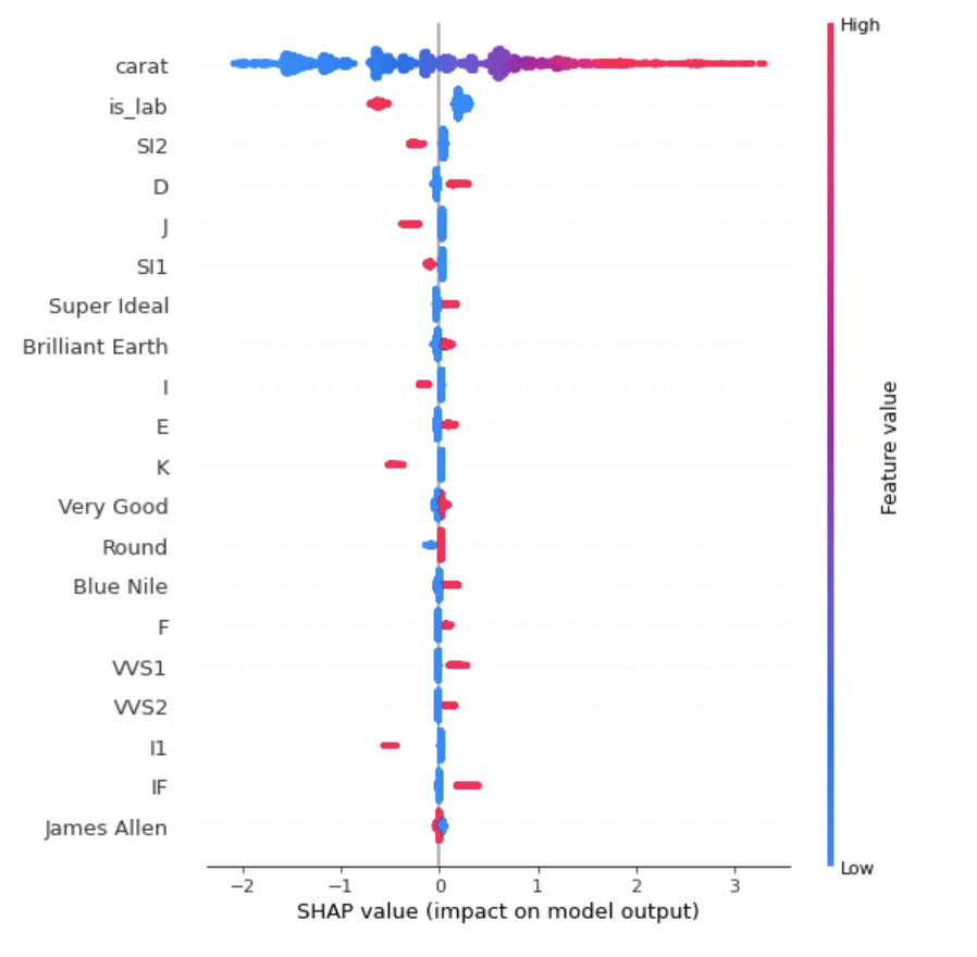
The chart above shows us the model’s calculated Shapley values for each feature and is meant to demonstrate feature importance. Before diving in more, one important aspect of understanding Shap is that Shapley values are derived in an additive nature. This means that a feature’s Shap value is calculated by comparing the predicted output to the score of the model prior to adding that feature. In a multivariate model all of our Shap values are additive on top of a baseline and this baseline is easiest to think of as the average value of the predicted dependent variable in our training dataset.

It shouldn’t be surprising to see that carat and whether or not a diamond is a lab diamond appear to be the two most important features to diamond price. Although it is interesting to see how much the model believes that K color and I1 inclusions contribute negatively to overall price.

To help understand Shap values a little better, let’s look at some individual examples. Below is a randomly selected diamond and a shap visualization of the models predicted score.

1
2
3
4
5
6
7
8
9

|                 |   131099 |
|:----------------|---------:|
| carat           |     0.62 |
| is_lab          |     1    |
| Emerald         |     1    |
| Super Ideal     |     1    |
| H               |     1    |
| VS1             |     1    |
| Brilliant Earth |     1    |

The baseline value that the model uses as a starting point is 7.694 representing the average of the natural log of the model’s predicted diamond price for the training data set. The Shapley values show each feature’s importance in the resulting predicted score for the diamond of 6.51. is_lab, carat, and the fact that the diamond is not a round cut but instead an emerald all contribute negatively to the predicted price relative to the base score. Interestingly, carat also contributes negatively to the base score but this is because our carat measurement of 0.62 is below the mean carat measurement for diamonds in our training set.

Shap is cool and all but why do this?

I had a couple of reasons why I wanted to build an XGBoost regression model and use Shap for interpretation beyond wanting very accurate predictions of diamond prices. Namely:

• I wasn’t convinced that assuming a linear relationship between diamond prices and our feature set was accurate
• I was fairly confident that there is “some” correlation between independent variables. For example, clarity might have a larger impact on price the larger a diamonds carat becomes. This intuitively makes sense but leads to problems with the coefficients of my linear model.
• An XGB model can help to find non-linearity and correlations between independent variables and Shap can be used to help to explain these phenomena.

The shap python package has a nifty method called dependence_plot that allows us to plot interactions between multiple independent variables and see the resulting changes in predicted Shap values. It also allows us through use of another method called shap_interaction_values to see the higher-order interaction effects between different independent variables and how these higher-order effects impacted predicted Shap values.

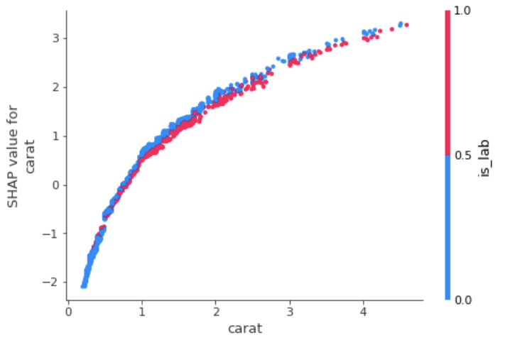
The plot above shows us Shap values for carat colored by whether or not a diamond is a lab diamond. Just looking at the graph, we can see that there is some small dispersion of predicted shap values for carat size based on whether or not the diamond is a lab diamond.

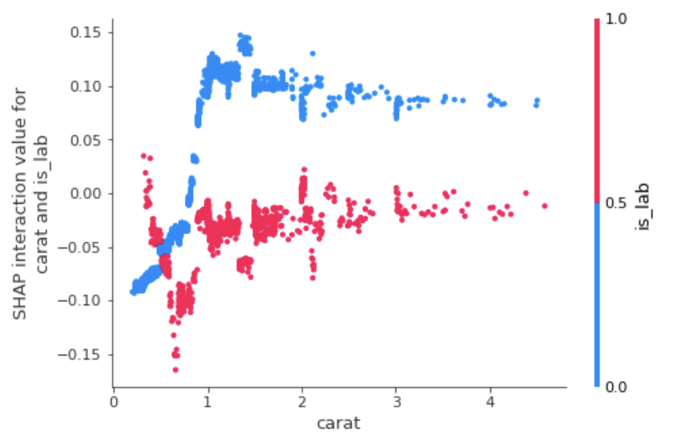
Plotting the interaction effects, we can see that the higher order impact of is_lab on carat is largest for carat values mid-way between 1 and 2. And at the minimum and maximum points of this chart, [-.15, .15], the interaction effects between carat and is_lab influence the predicted price of our diamond by roughly -14% to +16%.

Having looked at many of these interaction effects, I can tell you that there aren’t huge high-order effects in the XGB model. Thinking more about this, this feels that it makes intuitive sense given how well the linear model already performed in predicting diamond prices. All of this being said, some of the most interesting interaction effects for price conscious, prospective diamond buyers are going to be those related to the website selling the diamonds and diamond carat.

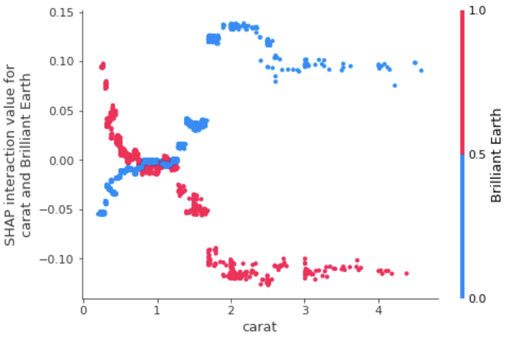
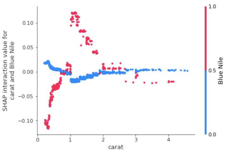
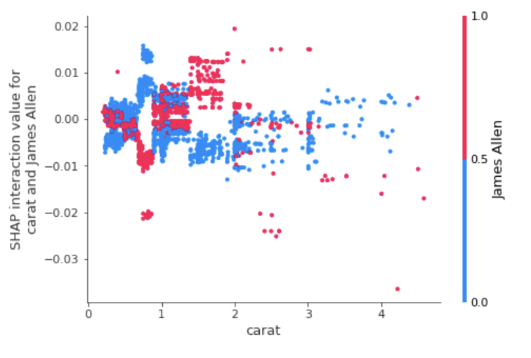
There aren’t any noticeable trends to higher order effects for James Allen diamonds. However, we can see clear trends for Blue Nile and Brilliant Earth diamonds with Brilliant Earth being slightly less expensive for diamonds greater than 1 carat and Blue Nile being less expensive for diamonds below 1 carat.

Conclusion

I know that for me personally, buying a diamond engagement ring was a nerve racking experience. My goal for this post was to give people a better sense of how diamonds are priced and what you might be getting for your money. I also hope that it was at least somewhat interesting. I wish you good fortune in your search and hope that I helped some way in some small bit.